Four homework assignments for the Microwave Devices course at the University of Padova, each with its own dimensions, loads and frequencies drawn from the student number. The method is the same every time: derive the structure analytically, compute its behaviour in MATLAB — ABCD matrices, S-parameters, frequency sweeps — and, where a full-wave simulation tells you something the formulas cannot, build it in CST Studio Suite and explain the difference.
Homework 01
One mode among dozens in a rectangular waveguide
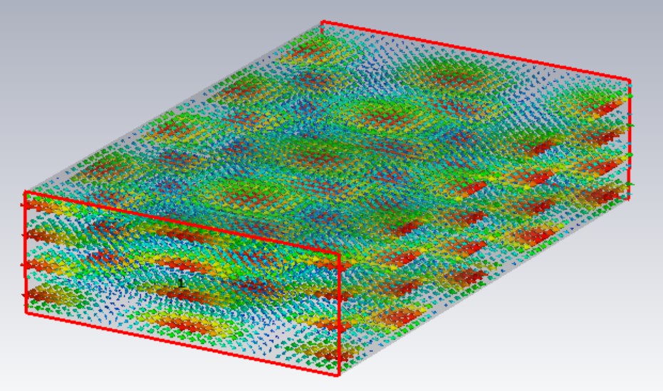
A 61.0 × 21.8 mm guide filled with a dielectric of εr = 3.9 carries dozens of modes before the one assigned, TE2,4, switches on at 14.15 GHz. Starting from its longitudinal magnetic field, the transverse components follow from Maxwell’s equations; CST then draws the same field, the currents on the walls and the power flow, and the MATLAB field maps line up with it. Around the mode come its propagation constant, phase and group velocity, modal impedance and guide wavelength from 1.2 to 1.8 times cut-off, and the delay it builds up over 90 m against two other modes. The last step is a modal filter: an electric wall placed across the electric field and a thin slot cut along the surface currents leave TE2,4 untouched while unwanted modes such as TE0,1 no longer propagate.
Homework 02
Matching 705 Ω to 50 Ω with a single stub
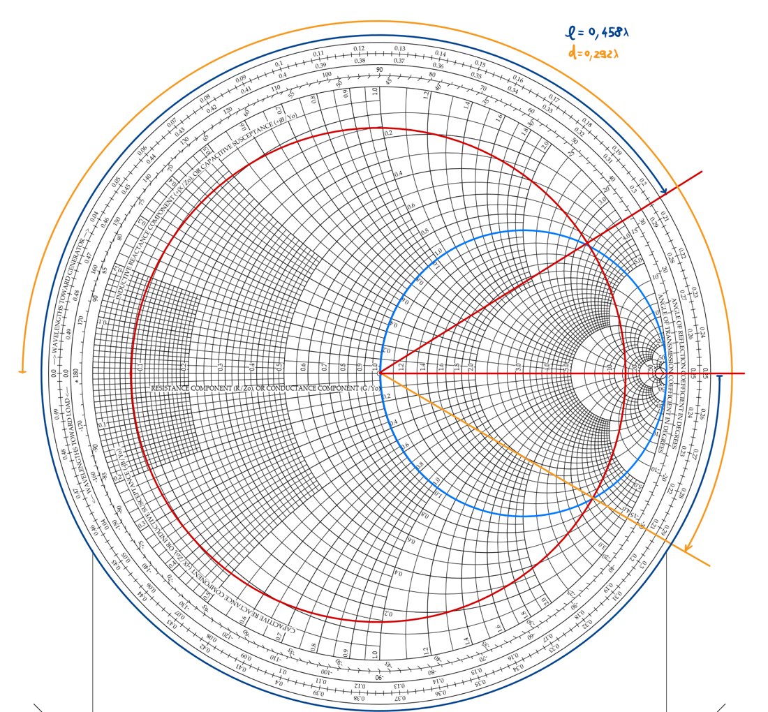
A 705 Ω load on a 50 Ω line at 2.365 GHz is fourteen times the line impedance. On the Smith chart the match comes out as a short-circuited shunt stub placed 0.292 λ from the load (37.0 mm) and 0.458 λ long (58.1 mm). The network is then rebuilt from ABCD matrices and swept from 0.2 to 1.8 times the design frequency: S-parameters, reflection coefficient, impedance, voltage, current and power on both sides of the stub, with reciprocity and losslessness checked numerically. Making the stub half a wavelength longer gives the same match at 2.365 GHz, since its input admittance repeats every λ/2 — but not the same response anywhere else.
Homework 03
A microstrip branch-line coupler, and why CST disagrees
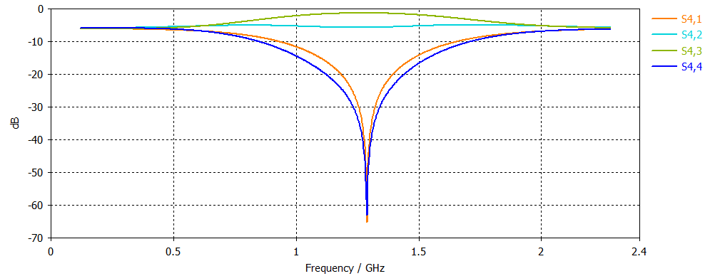
The coupler has 80 Ω ports, works at 1.2 GHz and has to send a quarter of the power, −6 dB, to its coupled port. An even/odd-mode analysis gives the two line impedances that make the input matched and the isolated port silent — 138.6 Ω and 69.3 Ω — and Hammerstad’s equations turn them into microstrip widths of 0.65 mm and 3.85 mm on a 3 mm substrate with εr = 3.5. In MATLAB the match and the isolation drop below −60 dB at 1.2 GHz, and twenty random ±5% errors on the two impedances show how quickly that depth is lost. Built in CST, the same layout centres about 7% high, near 1.29 GHz: the ideal-line model ignores the parasitic capacitance and inductance at the junctions where the narrow and wide lines meet, and the full-wave simulation does not.
Homework 04
From 11 MHz of bandwidth to almost 1 GHz
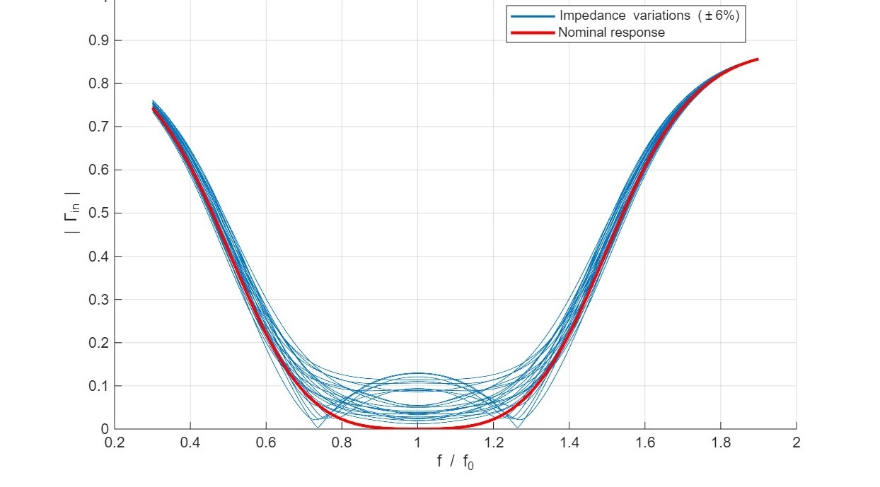
The same 705 Ω load, matched four more ways and judged on one number: how wide the band is where the reflection stays under 0.025. An L-section of lumped elements — 12.2 nH in series and 0.35 pF in shunt for the low-pass version — gives about 34 MHz, three times the single stub’s 11. A binomial, maximally flat transformer of quarter-wave sections changes the scale: with three sections the band is 653 MHz, with four 975 MHz, 41% of the centre frequency, computed exactly with ABCD matrices and compared with the small-reflection estimate. A tolerance run then gives each impedance of the four-section design a random ±6% error, 25 times: the response keeps its shape, but the ripple in the band rises to around 0.1, well above the 0.025 target — a broadband match is only as good as the impedances it is built from.
The four reports